Absence of Evidence in a Field of Sensors

Monitoring · July 28, 2026 · 9 min read

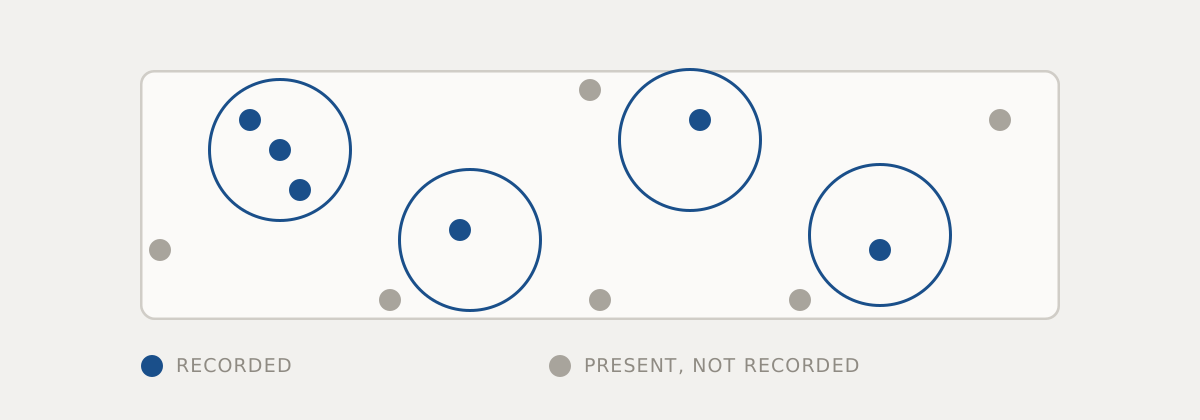
Monitoring programmes are commissioned to answer questions of the form is it working — is the population recovering, is the restoration establishing, is the mitigation doing what the consent required. Those are questions about states of the world.

What the equipment produces is something narrower: a list of times and places where a thing was noticed by an instrument. Detections, not states. The entire craft of ecological monitoring consists of getting from one to the other without pretending the gap is not there, and most disappointing monitoring programmes are ones where the gap was never modelled at all.

A record is a product of two things

Any detection requires the subject to be present and the survey to notice it. Those are separate probabilities, and only their product is observed.

The immediate consequence is that a bare map of records is at least as much a map of effort as a map of distribution. Where nothing was recorded, three explanations remain live: nothing was there, something was there and went unnoticed, or nobody looked properly. Nothing in the record itself distinguishes them.

This is why well-designed surveys have repeat structure — several visits, or several independent detectors, at the same place within a period over which the underlying state can be assumed not to change. Repeats are what make detection probability estimable, because a subject found on the third visit and missed on the first two supplies direct evidence about how often the method misses. Take the repeats out to save money and you have not bought a cheaper survey; you have bought a survey that cannot report uncertainty, which is a different product.

The same logic applies to continuous instruments. A camera or a recorder left in place is not exempt from detectability — it has a detection zone, a trigger threshold, a duty cycle and a set of conditions under which it fails to register something that walked past it. Continuous deployment gives you far more opportunities to detect. It does not give you certainty about the ones you missed.

Effort follows the road

Detection bias is rarely random, and its structure is usually logistical.

Sensors are placed where a vehicle can reach, where a permission exists, where the ground is firm enough to stand on, where the equipment will not be stolen. Repeat visits concentrate near the field station. Volunteer records cluster around footpaths and car parks and around the weekends. None of this is carelessness; it is what fieldwork costs. But it means the sampled subset of the landscape differs systematically from the landscape — typically towards edges, accessible habitat and disturbed ground.

Analysis can partially correct for this, provided the effort was recorded. Recording where, when and for how long you looked, including the occasions that produced nothing, is what makes correction possible. Zero-detection surveys are data. They are also the ones most likely to be dropped from a spreadsheet because they look empty.

A step in the series is usually a step in the instrument

Long-running sensor deployments accumulate a specific class of artefact, and it is easy to mistake for signal.

Sensors drift as they age and as they foul. Optical windows haze, membranes degrade, housings admit moisture, insects nest in inlets. Vegetation grows in front of a camera over a season and steadily reduces the detection zone, producing a smooth decline that looks exactly like a smooth decline in abundance. Batteries weaken and the duty cycle silently shortens. A microphone’s sensitivity changes and the effective detection radius changes with it, which changes the area being surveyed without changing anything visible in the data.

Then there are the deliberate changes. A firmware update alters a trigger threshold. A replacement unit is a newer model with different optics. A technician repositions a sensor by a few metres after a flood. Each is a sensible field decision and each introduces a discontinuity into a series that will later be analysed as though the method was constant.

The defensive practice is unglamorous and it works: treat instrument metadata as part of the dataset. Serial numbers, firmware versions, exact positions, maintenance events, cleaning, replacements, threshold settings — all timestamped in the same series as the observations. When a step change appears, the first question is what changed about the instrument, and that question should be answerable from the record rather than from someone’s memory of that summer.

Automated classification adds a second detection layer

Once detections are produced by a model rather than a person, there are two detectability problems stacked on each other: whether the sensor registered the event, and whether the classifier called it correctly.

Classifier performance is not a constant of the model. Recall and precision vary by species, by background noise, by season, by distance, by the acoustic or visual character of the specific site. A model that performs well on the data it was developed against can behave quite differently at a site with different ambient conditions — and the change is invisible, because the output format is identical. A drop in detections may mean fewer animals, or may mean the wind regime changed and the classifier’s recall fell with it.

This has a governance implication that is often missed: swapping in a better model mid-programme changes the survey protocol. The detection function has moved, so pre-change and post-change counts are not comparable without re-processing the archive under the new model. Keeping the raw audio, imagery or signal — not only the classified output — is what preserves that option. Deleting raw data to save storage is a decision to freeze your protocol permanently, and it is usually made by someone who does not know that is what they are deciding.

Validation should mirror deployment rather than the training set: a human-checked subsample from your sites, across your seasons, reported as error rates conditional on the conditions where they were measured.

Reporting in the units of the decision

The last failure is at the interface with whoever commissioned the work. A regulator, a landowner or a board is deciding something, and the decision has a threshold in it. A report that supplies a count, or a trend line, without any statement of what the method could and could not have detected, invites that threshold to be applied to a number that was never capable of supporting it.

The alternative is not hedging. It is being specific about the sensitivity of the method: what the survey would have detected had it been present, over what area, with what confidence, and what magnitude of change this design could distinguish from noise over this period. A programme that reports it could not have detected a change smaller than some amount has said something genuinely useful, and has protected itself from being quoted as evidence of stability.

Monitoring that cannot tell not there from not seen still produces tidy figures on a schedule. It just produces them at whatever rate the equipment happened to be working.